# import packages ----library(tidyverse) # data wrangling & viz (with {ggplot2})library(plotly) # JS plots!library(DT) # JS tables!library(leaflet) # JS maps!library(leaflet.extras) # leaflet add-ons!# reading in data ----1lobs <-readRDS(file = here::here("data", "lobsters.rds"))
1
RDS (R Data Serialization) is a data file format commonly used for saving R objects. RDS files are relatively small, take less time to import/export, and preserve data types and classes (e.g. factors and dates), eliminating the need to redefine data types after loading the file. We’ve done some pre-processing of the original/raw data and wrote it out as an .rds file (using saveRDS()) for us to use in this workshop.
1. Summarizing the data
# creating new data frame ----lobs_summary <- lobs %>%# calculate total lobster counts by protection status, site, & year (each point will represent lobster counts at a single site for each year from 2012-2018) ----group_by(protection_status, site, year) %>%# count the total number of lobsters summarize(n =sum(total_count))
2. plotly
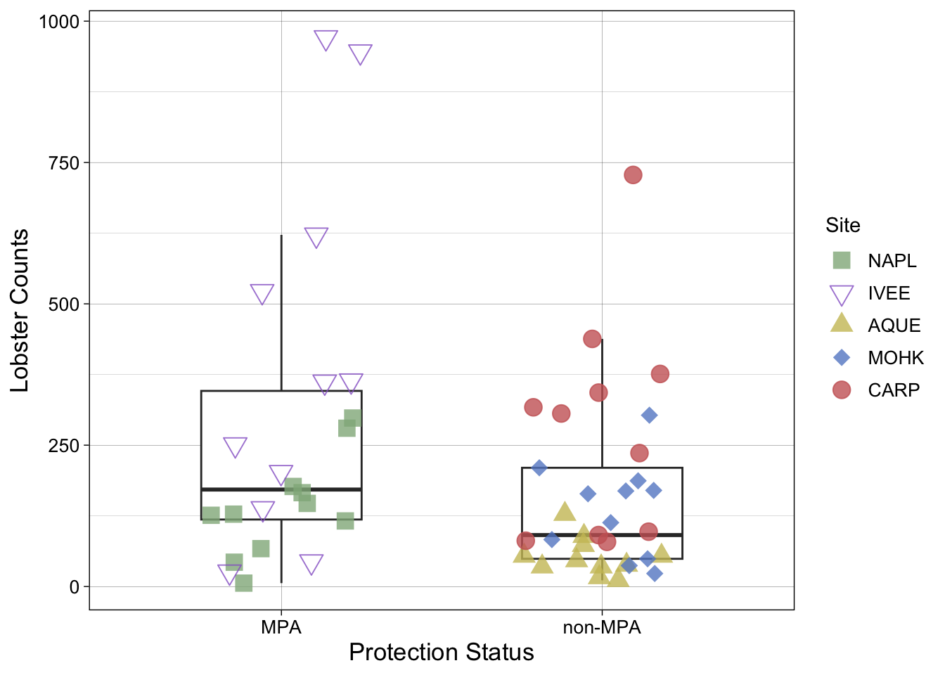
a. create a static plot
static <- lobs_summary %>%# create boxplot of mpa vs non-mpa lobster counts ----ggplot(aes(x = protection_status, y = n)) +# geoms: a boxplot and points with jitter ----geom_boxplot(width =0.5, outlier.shape =NA) +geom_point(aes(color = site, shape = site), size =4, alpha =0.8, # turn the points into a jitter (with a little more control than geom_jitter)position =position_jitter(width =0.25, height =0, seed =1)) +# update colors and shapes ----scale_color_manual(values =c("NAPL"="#91B38A", "IVEE"="#9565CC", "AQUE"="#CCC065", "MOHK"="#658ACC", "CARP"="#CC6565")) +scale_shape_manual(values =c(15, 25, 17, 18, 19)) +# update labels ----labs(x ="Protection Status",y ="Lobster Counts",color ="Site", shape ="Site") +# theme ----theme_linedraw() +theme(axis.text =element_text(size =10),axis.title =element_text(size =13),legend.text =element_text(size =10),legend.title =element_text(size =11))# print plot ----static
b. create an interactive plot
ggplotly(static) # ta-da!
c. create a better interactive plot
i. create a marker
# adding a column to lobs_summary ----lobs_summary_marker <- lobs_summary %>%# create a new column called "marker" ----mutate(marker =paste0("Site: ", site, "<br>","Year: ", year, "<br>","Status: ", protection_status, "<br>","Lobster count: ", n))
ii. make a new static plot with text = marker aesthetic argument
# creating a new static plot ----static_with_marker <- lobs_summary_marker %>%# create boxplot of mpa vs non-mpa lobster counts ----ggplot(aes(x = protection_status, y = n, text = marker, group = protection_status)) +# geoms: boxplot and jitter ----geom_boxplot(width =0.5, outlier.shape =NA) +geom_point(aes(color = site, shape = site), size =4, alpha =0.8, position =position_jitter(width =0.25, height =0, seed =1)) +# update colors and shapes ----scale_color_manual(values =c("#91B38A", "#9565CC", "#CCC065", "#658ACC", "#CC6565")) +scale_shape_manual(values =c(15, 25, 17, 18, 19)) +# update labels ----labs(x ="Protection Status",y ="Lobster Counts",color ="Site", shape ="Site") +# theme ----theme_linedraw() +theme(axis.text =element_text(size =10),axis.title =element_text(size =13),legend.text =element_text(size =10),legend.title =element_text(size =11))# printing the ggplot object will give you a scary warning - that's ok! ----static_with_marker
Warning: The following aesthetics were dropped during statistical transformation: text
ℹ This can happen when ggplot fails to infer the correct grouping structure in
  the data.
ℹ Did you forget to specify a `group` aesthetic or to convert a numerical
  variable into a factor?
iii. create plot with markers
# tooltip = "text" corresponds to the aes() text call from above!lobs_interactive <-ggplotly(static_with_marker, tooltip ="text") %>%# layout: most formatting goes here! ----layout(font =list(family ="Times"),# editing the marker/tooltip/hoverlabel hoverlabel =list(# editing the font: all goes in a list()font =list(family ="Times",size =13,color ="#FFFFFF",align ="left" ) ) )# print plot ----lobs_interactive
iv. doing things in plot_ly
plot_ly(# call the data ---- lobs_summary_marker,# axes ----x =~ protection_status,y =~ n,# type: plot_ly equivalent of "geom" ----type ="box",# show underlying data ----boxpoints ="all",# center points on boxplot ----pointpos =0,# control width of jitter ----jitter =0.25,# tooltip ----hoverinfo ="text", text =~ marker,# colors ----color =~ protection_status,colors =c("cornflowerblue", "darkgreen")) %>%layout(# global font option ----font =list(family ="Times", size =14),# changing axis labels xaxis =list(title =list(text ="Protection status")),yaxis =list(title =list(text ="Lobster count")),# editing the marker/tooltip/hoverlabel hoverlabel =list(# editing the font: all goes in a list()font =list(family ="Times",size =13,color ="#FFFFFF",align ="left" ) ) )
3. DT
a. create a basic interactive table
datatable(data = lobs)
b. customizing your DT
lobs_dt <-datatable(data = lobs, # make the column names nice ----colnames =c("Year", "Date", "Site", "Protection status", "Transect", "Replicate", "Size (mm)", "Count", "Latitude", "Longitude"),# column filters: sliders and drop down menus ----filter ="top", # extensions: lots of these! ----extensions =c("Buttons", "ColReorder"),# options ----options =list(# list 10 entries at oncepageLength =10, # automatically size columnsautoWidth =TRUE,# highlight entries that match search termsearchHighlight =TRUE,# allow regular expressions and case insensitive searchessearch =list(regex =TRUE, caseInsensitive =TRUE),dom ="Bfrtip",# buttons optionsbuttons =c("copy", "csv", "excel", "pdf", "print", "colvis"),# links to extension callcolReorder =TRUE)) %>%# styling cells: coloring site background ----formatStyle("site",# styleEqual allows matches to column contents ----backgroundColor =styleEqual(levels =list("NAPL", "IVEE", "AQUE", "MOHK", "CARP"),values =c("NAPL"="#91B38A", "IVEE"="#9565CC", "AQUE"="#CCC065", "MOHK"="#658ACC", "CARP"="#CC6565") ) )# print table ----lobs_dt
4. leaflet
a. some cleaning and filtering
# create df of unique sites ----sites <- lobs %>%select(site, protection_status, lat, lon) %>%distinct()# just mpa sites ----mpa <- sites %>%filter(protection_status =="MPA")# just non-mpa sites ----non_mpa <- sites %>%filter(protection_status =="non-MPA")
5. Prepare a report with your interactive visualizations!
Dynamic visualizations are particularly effective when embedded in reports – check out this fictitious report, created using both .qmd and .rmd files (for a side-by-side comparison):
While you may notice some feature and formatting differences between the two, both Quarto documents and R Markdown documents are effective tools for generating reproducible reports that combine prose, code, and outputs.